Marchenko-Pastur distribution
Here is a simple function to calculate the covariance matrix (NumPy has a built-in more sophisticated version):
def cv(a):
    "Covariance matrix"
    return numpy.matmul(a, a.transpose())/a.shape[1]
If we have some completely random data, e.g.:
a1=numpy.random.normal(size=(5,30))

The covariance matrix looks like:
cv(a1)
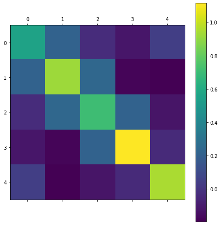
What are the eigen values of this matrix? We can obtain these using
the eigh numpy function:
ee, ev=numpy.linalg.eigh(cv(a1,a1))
In this case the ee array contains
array([0.50924555, 0.58887367, 0.94244866, 1.51785801, 1.80078024])
Obviously the eigen values are random just as the input matrix is, but what is their distribution? The answer is that it tends to the Marchenko-Pastur distribution:
\[P(\lambda) = \frac{ \sqrt{(\gamma_+ - \lambda)(\lambda-\gamma_-)} }{2 \pi \gamma \lambda}1_{x\in \left[ \gamma_-, \gamma_+\right]}\]where \(\gamma=n/p\), \(n\) is the number of rows in the matrix, \(p\) is the number of columns, \(\gamma_+ = (1+\sqrt{\gamma})^2\) and \(\gamma_- = (1-\sqrt{\gamma})^2\). If \(\gamma > 1\), i.e., there are fewer observations than variables in the input measurement matrix then \((1-1/\gamma)\) eigenvalues are zero. Here is a Python function describing the continuous part of the distribution:
def marchpast(l, g):
    "Marchenko-Pastur distribution"
    def m0(a):
        "Element wise maximum of (a,0)"
        return numpy.maximum(a, numpy.zeros_like(a))
    gplus=(1+g**0.5)**2
    gminus=(1-g**0.5)**2
    return numpy.sqrt(  m0(gplus  - l) *  m0(l- gminus)) / ( 2*numpy.pi*g*l)
Calculating the empirical eigenvalue distribution
Here is a simple demonstration in Python that the eigenvalues indeed tend to this distribution and which gives an idea of the inaccuracy of the distribution for finite sized matrices.
Since we are trying to find the distribution empirically we need generate a number of sample of covariance matrices as follows:
def randcv(n, p, s,
    t="N",
    f=None):
    """
    s lots of covariance matrices of random matrices of n x p shape

    t: N for normal, B for binary distribution [0,1]

    f: Filter. Z0 , Z1 for zscore on axis 0 or 1

    Returns  s x n x n array
    """
    r=[]
    for i in range(s):
        x=numpy.random.normal(size=(n,p))
        if t == "B":
            x=x>0.5
        if f == "Z0":
            x=scipy.stats.zscore(x, axis=0)
        elif f == "Z1":
            x=scipy.stats.zscore(x, axis=1)
        r.append(cv(x))
    return numpy.array(r)
And the following function can plot the empirical distribution:
def EE(a, gamma):
    "Calculate and show histogram of eigenvalues"
    ee, ev=numpy.linalg.eigh(a)
    nn, bb, patches=pyplot.hist(ee.ravel(),
                                bins="auto",
                                density=True)
    x=numpy.arange(bb[0], bb[-1], 0.003)
    pyplot.plot(x, marchpast(x, gamma))
    pyplot.ylim(top=nn[1:].max() * 1.1)
    pyplot.show()
Results
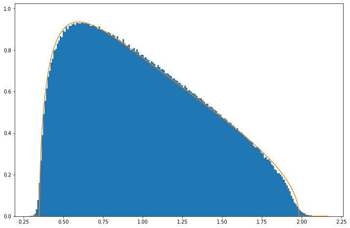
Below is what the empirical distribution looks like for the above case of a \(5\times30\) matrix, i.e., \(n=5\), \(p=30\). It can be seen that it follows roughly the expected Marchenko-Pastur but that some deviations are clear, especially that tails are more extended.
EE(randcv(5,30,50000, "N"), 5.0/30.)
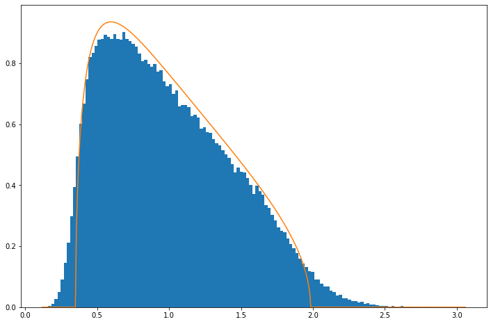
The reason for this is that Marchenko-Pastur is derived in limit \(n\rightarrow\infty\), \(p\rightarrow\infty\). The discrepancy is however not large and already by \(n=50\), \(p=300\) it is quite small:
EE(randcv(50,300,50000, "N"), 5.0/30.)
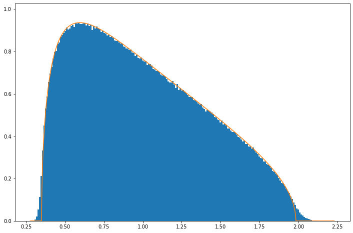
If you seeing a wide distribution of eighenvalues in your covariance matrices its unlikely due to be to the large \(n\), \(p\) limit!
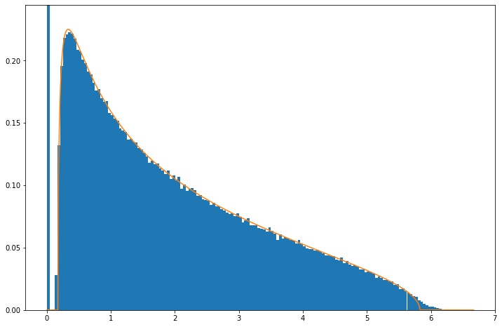
The same equation describes the continuous distribution of eigenvalues when \(\gamma>1\), but note that a large number of eigenvalues is zero to within numerical precision (the histogram’s y-axis is trunacated):
EE(randcv(100,50,5000, "N"), 10./5)
The same result applies for non-normal distributions. Here is an example for the binary distribution, i.e., where each element is drawn from \({0,1}\) and which we re-scale to have zero sample mean and unit sample variance in each column:
EE(randcv(50,300,50000, "B", "Z1"), 5.0/30.)
There is some evidence of systematic deviation from the distribution but again at level small enough not to matter in practice.