Efficient Hessian calculation with JAX and automatic forward- and reverse-mode differentiation
This is already fairly well documented in the JAX documentation but here it is with a moderately complex example that is not drawn from machine learning and some timings. The advantages of JAX for this particular example are:
-
Composable reverse-mode and forward-mode automatic differentiation which enables efficient Hessian computation
-
Minimal adjustment of NumPy/Python programs needed
-
Compilation via XLA to efficient GPU or CPU (or TPU) code
As you will see below the accelleration versus plain NumPy code is about a factor of 500!
Introduction
The Hessian matrix is the matrix of second derivatives of a function of multiple variables:
\[\mathbf H f(x_1\cdots x_n) = \begin{bmatrix} \dfrac{\partial^2 f}{\partial x_1^2} & \dfrac{\partial^2 f}{\partial x_1\,\partial x_2} & \cdots & \dfrac{\partial^2 f}{\partial x_1\,\partial x_n} \\[2ex] \dfrac{\partial^2 f}{\partial x_2\,\partial x_1} & \dfrac{\partial^2 f}{\partial x_2^2} & \cdots & \dfrac{\partial^2 f}{\partial x_2\,\partial x_n} \\[2ex] \vdots & \vdots & \ddots & \vdots \\[2ex] \dfrac{\partial^2 f}{\partial x_n\,\partial x_1} & \dfrac{\partial^2 f}{\partial x_n\,\partial x_2} & \cdots & \dfrac{\partial^2 f}{\partial x_n^2} \end{bmatrix}\]where \(f\) is a function of the \(n\) variables \(x_1\cdots x_n\). Since the matrix is symetric there is \(\frac{n(n+1)}{2}\) elements of Hessian to compute. Where a finite-difference method is used to compute the Hessian and \(n\) is large, the computation can become prohibitetively expensive.
Uses of the Hessian matrix
Most frequently cited use of the Hessian is in optimisation in Netwon-type methods (see Wikipedia ). The expense of computing it however means Quasi-Netwon methods are often used, where the Hessian is estimated rather than computed. Much more efficient Hessian matrix computation makes true Netwon methods tractable for a wide range of problems1.
Another application is calculation of the Fischer information matrix and the Cramér–Rao bound by calculating the Hessian of negative log-likelihod. This in turn allows estimation of variance of parameters when using maximum likelihood.
Example
As an example I am using a maximum likelihood calculation of fitting a simple model to two-dimensional raster observations (i.e., a monochromatic image).
The model2 is a two dimensional Gaussian:
\[G(x, y; \left[ x_0, y_0, a, \sigma, \rho, \delta \right] ) = a \exp{\left( \frac{-1}{ 2 \sigma^2 \left[ r^2 + \rho dx dy +\delta(dx^2-dy^2) \right]}\right)}\]where \(dx=(x-x_0)\), \(dy=(y-y_0)\) and \(r^2=dx^2 + dy^2\).
The Python code is straightforward:
def gauss2d(x0, y0, amp, sigma, rho, diff, a):
    """
    Sample model: Gaussian on a 2d plane
    """
    dx=a[...,0]-x0
    dy= a[...,1]-y0
    r=np.hypot(dx, dy)
    return amp*np.exp(-1.0/ (2*sigma**2) * (r**2 +
                                            rho*(dx*dy)+
                                            diff*(dx**2-dy**2)))
Likelihood
Very often the nest step would be to assume that observational uncertainty is normally distributed. This has a deep computational advantage3 but is however often not really the case as the prelevance of various attempts to clean the observed data before it is put into maximum likelihood analysis shows.
For this example I’ll instead assume that the uncertainty is distributed with the Cauchy distribution. The wider tails of this distribution means a maximum likelihood solution will be far less affected by a few outlier points.
The Python is simple:
def cauchy(x, g, x0):
    return 1.0/(numpy.pi * g) * g**2/((x-x0)**2+g**2)

def cauchyll(o, m, g):
    return -1 * np.log(cauchy(m, g, o)).sum()
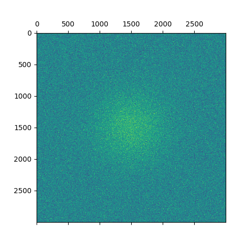
Observed data
I will use a simulated data set instead of an observation: a \(3000\times3000\) image with a Gaussian source in the middle and normally distributed noise:
Putting it together and applying JAX
Applying JAX to this non-trivial NumPy is extremely simple. It consists of :
- Using
jax.numpymodule instead of the standardnumpy - Decorating functions with
@jit - Calculating the Hessian by first doing reverse-mode and then forward-mode differentiation
Overal the number of changes is very small and it is quite practical to maintain a code-base which can be switched between numpy and JAX without modifications.
The main part of the program looks like this:
import jax.numpy as np
from jax import grad, jit, vmap, jacfwd, jacrev


@jit
def gauss2d(x0, y0, amp, sigma, rho, diff, a):
    """
    Sample model: Gaussian on a 2d plane
    """
    dx=a[...,0]-x0
    dy= a[...,1]-y0
    r=np.hypot(dx, dy)
    return amp*np.exp(-1.0/ (2*sigma**2) * (r**2 +
                                            rho*(dx*dy)+
                                            diff*(dx**2-dy**2)))

def mkobs(p, n, s):
    "A simulated observation"
    aa=numpy.moveaxis(numpy.mgrid[-2:2:n*1j, -2:2:n*1j], 0, -1)
    aa=np.array(aa, dtype="float64")
    m=gauss2d(*p, aa)
    return aa, m + numpy.random.normal(size=m.shape, scale=s)

@jit
def cauchy(x, g, x0):
    return 1.0/(numpy.pi * g) * g**2/((x-x0)**2+g**2)

@jit
def cauchyll(o, m, g):
    return -1 * np.log(cauchy(m, g, o)).sum()

def makell(o, a, g):
    def ll(p):
        m=gauss2d(*p, a)
        return cauchyll(o, m, g)
    return jit(ll)

def hessian(f):
    return jit(jacfwd(jacrev(f)))
The measurement of timings was done as follows:
# Calculate the hessian around this point, which by design is the
# most-likely point
P=np.array([0.,0., 1.0, 0.5, 0., 0.], dtype="float64" )

a, o = mkobs( P, 3000, 0.5)
ff=makell(o, a, 0.5)
hf=hessian(ff)
ndhf=nd.Hessian(ff)

# JIT warmup call. Smallish effect if number is large in timeit
hf(P).block_until_ready()

print("Time with JAX:", timeit.timeit("hf(P).block_until_ready()", number=10, globals=globals()))
print("Time with finite diff:", timeit.timeit("ndhf(P)", number=10, globals=globals()))
How efficient?
Running this Intel CPU (no GPU) I get following timings for 10 runs
using timeit:
- Time with JAX and automatic differentiation: 16s
- Time with JAX function valuation and finite-difference differentiation (with Numdifftools) : 891s
- Time with plain numpy and numerical differentiation (with Numdifftools): 9900s
So impressively there is a \(\times 500\) reduction in run-time! Note that this is a fairly large problem where the JIT costs are well amortized – the performance would not be this good for scattered small one-off problems. The improvement in performance can broken down as a \(\times 50\) gain due to automatic-differentiation and \(\times 10\) gain due to fusion and compilation using XLA.
Footnotes
-
Quasi-Netwon methods have some intrinsic advantages so even with efficient Hessian matrix they could be competitive. So the choice of algorithm probably needs to be considered on a case-by-case basis. ↩
-
This not an often used parametrisation but it is useful because the azimuthally independent dimensional width \(\sigma\) is a separate parameter from the squashedness of the Gaussian in the + and X directions which are given by dimensionless parameters \(\rho, \delta\) ↩
-
Because the log-likehood will correspond to sum of squares of deviations of the model from observations – hence the traditional least-squares methods ↩