Principal Component Analysis in Excel
If you like to fit straight lines to two dimensional datasets, you’ll probably like doing Principal Component Analysis (PCA) to multidimensional ones. It can be seen as a generalisation specifically of orthogonal distance regression to higher dimensions. There is a nice presentation in the booklet Dimension Reduction: A Guided Tour, by Burges. A nice further discussion is also presented at this blog.
In many cases it is useful to keep a keen eye on the actual data used
in PCA, and in this case Excel is a great tool. It is then convenient
to the PCA from within which fortunately can be done extremely easily
with python, the scikit-learn python package and
xlwings to connect excel to python.
You may also be interested on in-depth data-analysis using tools including Excel appearing here.
Setup
If you already have Python and/or xlwings installed you can skip the following two sub-sections.
Installing python
I install the plain Windows installer, which you can get straight from python.org :
https://www.python.org/ftp/python/3.9.5
Select the option to add Python environment variables.
See the post on installing Python
Installing xlwings
There are comprehensive instructions on the xlwings website for the package and specifically for the addin. In brief, it consists of:
Installing the xlwings package via pip:
pip install xlwings
xlwings addin install
And then changing a trust option in Excel by navigating “File -> Options -> Trust Center -> Trust Center Settings -> Marco Settings -> (Enable) Trust access to VBA project object model”
Preparing Python for PCA
I use the PCA implementation in scikit-learn, hence we need to
installed this package:
pip install scikit-learn
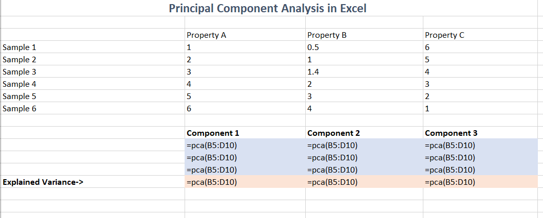
Connecting this with Excel is then trivial: Python code below, saved
with the same name as your spreadsheet (but “.py” suffix) will make
available a new function =pca() which computes the principal
component analysis:
import numpy
from sklearn import decomposition

import xlwings as xw

@xw.func
@xw.arg("d", numpy.array, ndim=2)
@xw.ret(expand="table")
def pca(d):
    p=decomposition.PCA(d.shape[1])
    x=p.fit(d)
    return numpy.vstack([x.components_.transpose(), x.explained_variance_])
Example in use
An example of all this in action is below. Some things to remember:
- Always look at the explained variance
- Reduce the display precision to appropriate level
- If you project to do a 2d scatter plot, remember that a (hyper)-plane will project to a line, and you can see the same line in lots of different projections
- If you do projections of data, remember that even if any observational noise is uncorrelated between the properties, it will be correlated between projections
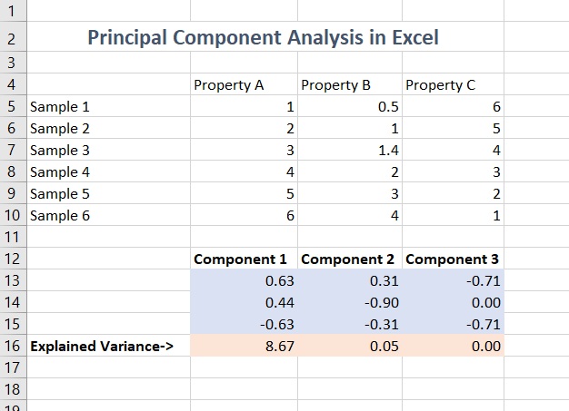
The formula used to produce this result is simply a call to the
=pca() function:
Enjoy finding answers in your data!
You may also be interested on in-depth data-analysis using tools including Excel appearing here. See for example this article on Principal Component Analysis of Gilt Spot Yield Curves.